Flight Price Prediction

Project Overview
This project is divided into multiple deliveries, each focusing on different aspects of data mining, from data selection and exploration to migration, modeling, and dashboard presentation.
Our Team
 |
 |
|---|---|
| Data engineer Shadia Jafaar is a student at the Universidad del Norte in the systems engineering program in seventh semester, graduated from Biffi La Salle school in 2020, his area of interest is focused on the management of big data, cloud computing and technology sales. He has knowledge in various programming languages but focuses mainly on python and sql for data manipulation. He is passionate about sports and learning new things. The role he will develop in the team will be a data engineer and he will be one of the people in charge of data manipulation and data cleaning. | Data engineer Yuli Meza Barros, 22 years old student on 9th-semester of systems engineering at Universidad del Norte, completed her studies at Nuestra Señora de Lourdes School in 2019. With a profound interest in cybersecurity, she demonstrates proficiency in Java and Python programming languages. Her fascination extends to data analytics, showcasing a versatile skill set. In the team, Yuli plays a vital role as a data engineer, specializing in meticulous data manipulation and cleaning processes Her diverse interests and skills contribute to the dynamic and collaborative environment within the team. |
 |
 |
|---|---|
| Backend engineer David Meza, a eighth-semester student at Universidad del Norte, graduated from INEDINSA, has a keen interest in backend development, databases, and distributed systems. With a passion for crafting robust solutions and learning from existent ones. Outside of the tech realm, David enjoys expressing his creativity through playing the piano and has a particular fondness for languages. | Frontend engineer Julián Coll, a seventh-semester systems engineering student at Universidad del Norte, graduated from I.E.T.C. Francisco Javier Cisneros at 2020, who has some experience in backend development and database management. Proficient in Python, SQL, and relational databases. Dedicated to designing efficient systems to meet project goals. I am responsible for the visual part of the project emphasizing the user experience. |
Delivery 1: Data Selection
Due Date: 16/08/2024
Dataset Chosen
The dataset selected for the “Flight Price Prediction” project comprises 300,261 datapoints and 11 features. This data was scraped from the “Ease My Trip” website, covering flight bookings between India’s top 6 metro cities over a 50-day period in early 2022.
Dataset Description
Features
- Airline: The carrier operating the flight. Helps analyze pricing strategies of different airlines.
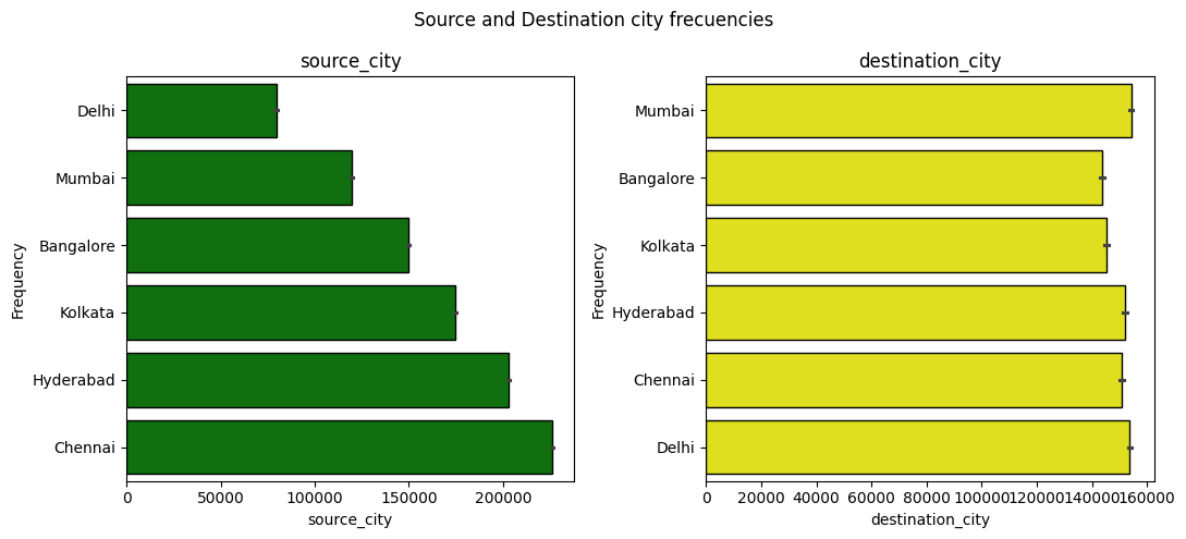
- Source City: The city from which the flight departs. Allows examination of regional price variations.
- Destination City: The city where the flight lands. Helps understand price differences based on destination demand.
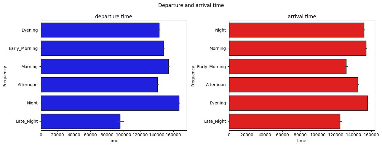
- Departure Time: The scheduled time when the flight departs. Useful for analyzing how different times of day affect prices.
- Arrival Time: The scheduled time when the flight arrives. Helps in understanding how arrival schedules influence pricing.
- Ticket Class: The class of the ticket (e.g., Economy, Business). Allows comparison of pricing between different ticket classes.
- Days Left: The number of days remaining until departure. Critical for analyzing the impact of booking timing on prices.
Data Quality and Coverage
- Data Completeness: The dataset is extensive, but may have missing values or incomplete records, especially for features like departure and arrival times.
- Data Accuracy: The accuracy is based on the scraping process and source reliability. Some discrepancies in ticket prices and times may exist.
Justification
The chosen dataset is well-suited for analyzing and predicting flight prices due to its comprehensive nature and relevance to the project goals.
Potential Insights
- Price Variation by Airline: Analyze how different airlines set their prices, revealing competitive pricing strategies.
- Impact of Booking Time: Investigate how the number of days left until departure affects ticket prices.
- Effect of Departure and Arrival Times: Examine how different flight times impact prices.
- Class-Based Price Differences: Compare pricing between economy and business class tickets.
Expanded Methodology
- Data Preprocessing: Clean the dataset by addressing missing values, encoding categorical variables, and scaling continuous variables if necessary.
- Exploratory Data Analysis (EDA): Utilize statistical summaries and visualizations to understand feature distributions and relationships.
- Statistical Analysis: Perform correlation analysis and ANOVA tests to understand feature impacts on pricing.
- Predictive Modeling: Develop linear regression models and explore advanced techniques like decision trees and ensemble methods.
- Model Evaluation: Use cross-validation and performance metrics (MAE, RMSE) to assess and refine models.
Relevance
The dataset aligns closely with the project goals and research questions. Here’s how each feature addresses the research questions:
- Airline: Helps in understanding price variations by comparing how different airlines price their tickets under similar conditions. This feature can reveal competitive pricing strategies and brand-specific pricing patterns.
- Days Left: Allows analysis of how booking timing influences ticket prices. By examining how prices change as the departure date approaches, we can identify trends in pricing strategies related to booking timing.
- Departure and Arrival Times: Facilitates examination of how different flight times impact prices. This helps understand if flights during peak hours or specific times of the day are priced differently.
- Ticket Class: Provides insights into class-based pricing differences. By comparing economy and business class prices, we can determine the pricing strategies for different levels of service and amenities.
Examples of Similar Studies
- Dynamic Pricing in Airlines: A study by Zhang et al. (2021) used similar datasets to explore dynamic pricing models in the airline industry, revealing how factors like booking time and demand affect ticket prices. They applied machine learning techniques to predict price changes and optimize revenue management.
- Airline Pricing Strategies: Chen and Yang (2019) conducted research on airline pricing strategies using datasets with features like departure times and ticket classes. Their study focused on how airlines adjust prices based on demand, competition, and time of booking.
- Impact of Departure Times on Pricing: Research by Hsu and Tsai (2020) examined how departure and arrival times influence flight prices. Their analysis highlighted price patterns associated with different times of day and peak travel periods, using data similar to what is available in this dataset.
Delivery 2: Data Selection
Due Date: 13/09/2024
Exploratory Data Analysis (EDA)
Data Overview
The dataset used for flight price prediction consists of 300,153 observations and 12 variables. Below is a summary of the dataset’s key details:
- Total rows (observations): 300,153
- Total columns (variables): 12
- Dataset size: 27.5 MB
Variable Description:
| Column | Data Type | Description |
|---|---|---|
| Unnamed: 0 | int64 | Index column (not used in analysis) |
| airline | object | Airline operating the flight |
| flight | object | Flight identification |
| source_city | object | City from which the flight departs |
| departure_time | object | Scheduled flight departure time |
| stops | object | Number of stops during the flight |
| arrival_time | object | Scheduled flight arrival time |
| destination_city | object | Destination city of the flight |
| class | object | Ticket class (e.g., economy, business) |
| duration | float64 | Duration of the flight in hours |
| days_left | int64 | Days left until flight departure |
| price | int64 | Flight ticket price (in local currency) |
Data Types:
- Numerical variables (4):
Unnamed: 0,duration,days_left,price - Categorical variables (8):
airline,flight,source_city,departure_time,stops,arrival_time,destination_city,class
Exogenous Repositories
The following external data could enhance the accuracy of flight price predictions:
1. Tourism Demand or Seasonality Data
This data can help explain price variations based on flight destinations.
-
Relevance: Tourism demand fluctuates based on seasons and events, affecting flight prices. Prices tend to increase during peak seasons and decrease during off-seasons.
-
Potential Impact:
- Improved price prediction by identifying demand spikes.
- Isolate seasonal effects to better understand price fluctuations unrelated to other factors.
2. Fuel Price Data
Fuel price data reflects the operational costs of airlines.
-
Relevance: Fuel costs directly influence airline operational expenses, which in turn affect ticket prices.
-
Potential Impact:
- Predict price changes based on fluctuations in fuel costs.
- Identify long-term trends that could impact flight prices.
Incorporating these additional datasets will allow for more accurate price predictions and a better understanding of the factors driving flight price variations.
Data Visualization
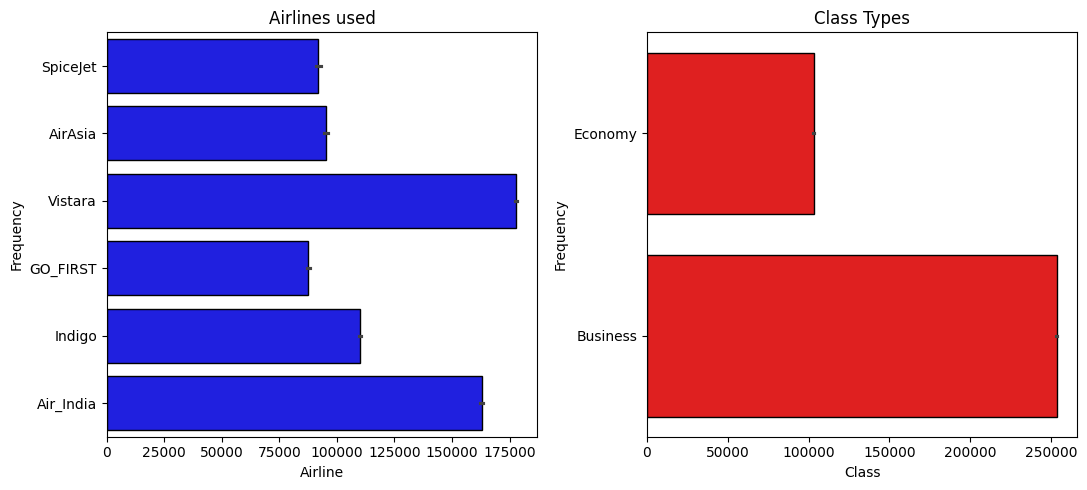
First, let’s look at the proportion of occurrences for some interesting categorical variables:
Next, let’s examine the distribution of the numerical variables in our dataset:
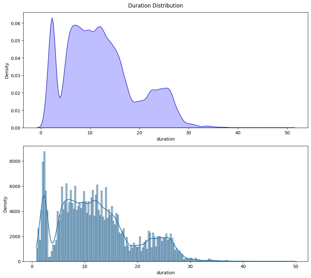

Now, let’s check for outliers in the numerical columns:
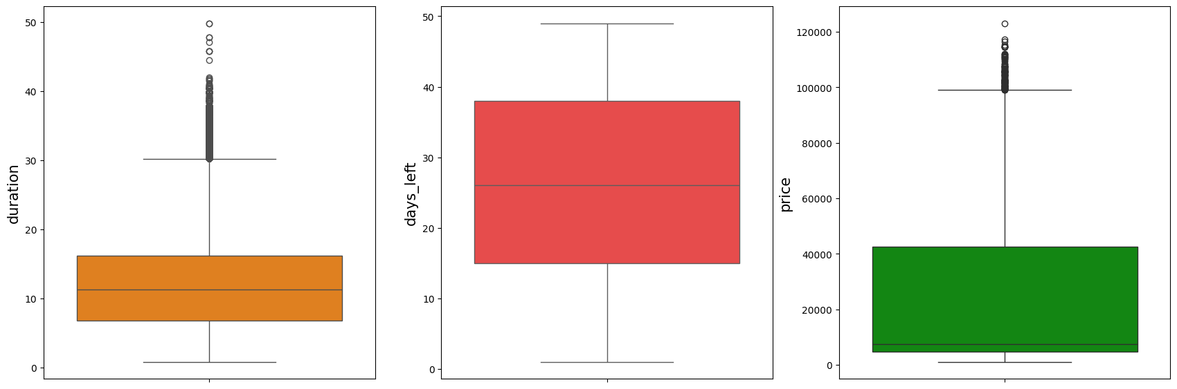
We can observe that there are outliers in the duration and price columns.
Data Cleaning
Null Values Check
We verified that there are no null values across any of the columns in the dataset. All columns were complete.
Duplicate Values Check
We confirmed that there are no duplicate records in the dataset, ensuring the integrity of the data.
Removing Unnecessary Columns
The Unnamed column, which was irrelevant to the analysis, was removed for clarity.
Unique Values in Columns
The dataset contains the following number of unique values in each column:
- Airline: 6 unique values
- Flight: 1561 unique values
- Source City: 6 unique values
- Departure Time: 6 unique values
- Stops: 3 unique values
- Arrival Time: 6 unique values
- Destination City: 6 unique values
- Class: 2 unique values
- Duration: 476 unique values
- Days Left: 49 unique values
- Price: 12,157 unique values
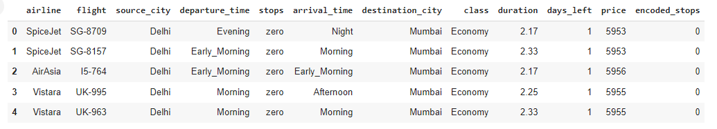
Encoding Categorical Data
We converted the categorical variable stops into numerical format to facilitate modeling.
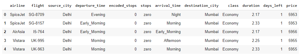
Reordering Columns
The encoded_stops column was moved to a more logical position for easier analysis.
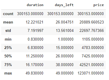
Statistical Summary of Numerical Columns
Below is the statistical description of the numeric columns in the dataset, showing key metrics such as mean, standard deviation, minimum, and maximum values.
Data Imputation
In this dataset, no missing values were found, as confirmed by the earlier data exploration step. Therefore, no data imputation was necessary.
Common Imputation Techniques
If missing values were present, the following imputation techniques could have been considered:
- Mean/Median Imputation: For numerical variables, imputing missing values with the mean or median is common, depending on whether the data is skewed.
- Mode Imputation: For categorical variables, the most frequent value (mode) could be used to replace missing values.
- Forward/Backward Fill: For time series data, missing values can be filled by propagating previous or next valid values.
- K-Nearest Neighbors (KNN) Imputation: This technique finds the nearest neighbors based on a distance metric and imputes missing values by averaging the values of these neighbors.
Justification
Since the dataset is complete and free from missing data, none of these techniques were required in this project. This ensures that no bias was introduced through the imputation process.
Delivery 3: Data Migration to BigQuery and Model Preparation
Due date: 18/10/2024
Data Migration:
In order to upload the Pandas dataframes used to training our model, we first had to create a new Google Cloud Project. Within it, we also created a new dataset, which would contain the previously mentioned dataframes.
Once everything was set and ready, we used pandas_gbq.to_gbq() function in Google Colab to upload all the files into the newly created dataset.
However, for this method to work, we first needed a way to access GCP within Google Colab. So we created a service account and generated a new JSON key, which we granted the Owner role for now.
After using the key in the pandas_gbq.to_gbq() function, we were able to upload the neccesary files to GCP.
Chosen Model
Ridge regression is a type of linear regression that includes a regularization term to penalize the magnitude of the coefficients of the model. It adds an L2 regularization term to the cost function, which is the sum of the squared coefficients. This regularization term helps to prevent the model from overfitting by shrinking the coefficients, which means it reduces the model’s complexity without affecting its predictive power significantly.
Training Process
The first step in building a machine learning model is to divide the data into training and testing sets. This is done to evaluate the model’s performance on unseen data and prove the generalization ability of the model. For the Ridge model predicting flight prices, the data would be split into a training set 80% of data and a test set (the remaining 20%).
Training set:
Used to train the model, where the model learns the relationship between features and the target variable (flight price).
Test set:
Used to evaluate how well the model generalizes to new data. It helps in assessing the model’s prediction accuracy and detecting overfitting or underfitting.
For this project, we used the train_test_split function. It consists of randomly dividing the original dataset into two parts: a training set and a test set, using a specified proportion (e.g., 70% for training and 30% for testing).
Hyperparameter Tunning:
Machine learning models often include hyperparameters. Ridge regression includes a hyperparameter called the regularization parameter (alpha), which controls the complexity of the model. However, finding the optimal value is not trivial, so we use a grid search to achieve this. This method systematically tests a range of possible values for the hyperparameter.
First, we define a set of candidate values for alpha (e.g., [0.01, 0.1, 1, 10, 100]). The algorithm evaluates the model’s performance for each value and selects the one that maximizes the metric of interest (in this case, we chose R²)
Cross validation:
Cross-validation helps to ensure that the model’s performance is evaluated more robustly. Using cv=5 means that the data is split into 5 “folds”:
The data is divided into five equal parts.
In each iteration, four parts are used for training, and one part is used for validation.
This process repeats five times, with each fold serving as the validation set once.
After the five iterations, the results are averaged to get a more reliable estimate of the model’s performance.
Metrics and Results Analysis:
-
Mean Squared Error (MSE): indicates the average squared difference between the predicted and actual flight prices. Since MSE squares the differences between the predicted and actual values, the resulting value is in squared units. This makes it less interpretable in the context of the original units.
-
Root Mean Squared Error (RMSE): gives an estimate of the standard deviation of the prediction errors in the original units (e.g., dollars). This suggests that, on average, the model’s predictions are off by approximately $6814.
-
Mean Absolute Error (MAE): shows the average absolute difference between the predicted and actual flight prices. The given value indicates that the Ridge regression model’s predictions for flight prices are, on average, $4500.71 away from the actual prices.
-
R² Score: indicates that the model explains about 91% of the variance in the flight prices. This suggests a strong fit, meaning the model captures most of the variability in the data.
-
Best Hyperparameters: The optimal value for the regularization parameter alpha was found to be 0.1. This indicates a moderate level of regularization, which helps prevent overfitting while still fitting the data well.